It is based on some notion of "distance" (the inverse of similarity) between data points and use that to identify data points that are close-by to each other. In the following, we discuss some very basic algorithms to come up with clusters, and use R as examples.
K-Means
This is the most basic algorithm
- Pick an initial set of K centroids (this can be random or any other means)
- For each data point, assign it to the member of the closest centroid according to the given distance function
- Adjust the centroid position as the mean of all its assigned member data points. Go back to (2) until the membership isn't change and centroid position is stable.
- Output the centroids.
K-Means is highly scalable with O(n * k * r) where r is the number of rounds, which is a constant depends on the initial pick of centroids. Also notice that the result of each round is undeterministic. The usual practices is to run multiple rounds of K-Means and pick the result of the best round. The best round is one who minimize the average distance of each point to its assigned centroid.
Here is an example of doing K-Means in R
> km <- kmeans(iris[,1:4], 3)
> plot(iris[,1], iris[,2], col=km$cluster)
> points(km$centers[,c(1,2)], col=1:3, pch=8, cex=2)
> table(km$cluster, iris$Species)

setosa versicolor virginica
1      0         48        14
2     50          0         0
3      0          2        36

Hierarchical Clustering
In this approach, it compares all pairs of data points and merge the one with the closest distance.
- Compute distance between every pairs of point/cluster. Compute distance between pointA to pointB is just the distance function. Compute distance between pointA to clusterB may involve many choices (such as the min/max/avg distance between the pointA and points in the clusterB). Compute distance between clusterA to clusterB may first compute distance of all points pairs (one from clusterA and the other from clusterB) and then pick either min/max/avg of these pairs.
- Combine the two closest point/cluster into a cluster. Go back to (1) until only one big cluster remains.
Here is an example of doing hierarchical clustering in R
> sampleiris <- iris[sample(1:150, 40),]
> distance <- dist(sampleiris[,-5], method="euclidean")
> cluster <- hclust(distance, method="average")
> plot(cluster, hang=-1, label=sampleiris$Species)

Fuzzy C-Means
Unlike K-Means where each data point belongs to only one cluster, in fuzzy cmeans, each data point has a fraction of membership to each cluster. The goal is to figure out the membership fraction that minimize the expected distance to each centroid.

The algorithm is very similar to K-Means, except that a matrix (row is each data point, column is each centroid, and each cell is the degree of membership) is used.
- Initialize the membership matrix U
- Repeat step (3), (4) until converge
- Compute location of each centroid based on the weighted fraction of its member data point's location.

- Update each cell as follows


Here is an example of doing Fuzzy c-means in R
> library(e1071)
> result <- cmeans(iris[,-5], 3, 100, m=2, method="cmeans")
> plot(iris[,1], iris[,2], col=result$cluster)
> points(result$centers[,c(1,2)], col=1:3, pch=8, cex=2)
> result$membership[1:3,]
         1           2         3
[1,] 0.001072018 0.002304389 0.9966236
[2,] 0.007498458 0.016651044 0.9758505
[3,] 0.006414909 0.013760502 0.9798246
> table(iris$Species, result$cluster)
        1  2  3
setosa      0  0 50
versicolor  3 47  0
virginica  37 13  0

Multi-Gaussian with Expectation-Maximization
Generally in machine learning, we will to learn a set of parameters that maximize the likelihood of observing our training data. However, what if there are some hidden variable in our data that we haven't observed. Expectation Maximization is a very common technique to use the parameter to estimate the probability distribution of those hidden variable, compute the expected likelihood and then figure out the parameters that will maximize this expected likelihood. It can be explained as follows ...
 Now, we assume the underlying data distribution is based on K centroids, each a multi-variate Gaussian distribution. To map Expectation / Maximization into this, we have the following.
 The order of complexity is similar to K-Means with a larger constant. It also requires K to be specified. Unlike K-Means whose cluster is always in circular shape. Multi-Gaussian can discover cluster with elliptical shape with different orientation and hence it is more general than K-Means.
Here is an example of doing multi-Gaussian with EM in R
> library(mclust)
> mc <- Mclust(iris[,1:4], 3)
> plot(mc, data=iris[,1:4], what=c('classification'),
       dimens=c(3,4))
> table(iris$Species, mc$classification)

 1  2  3
setosa     50  0  0
versicolor  0 45  5
virginica   0  0 50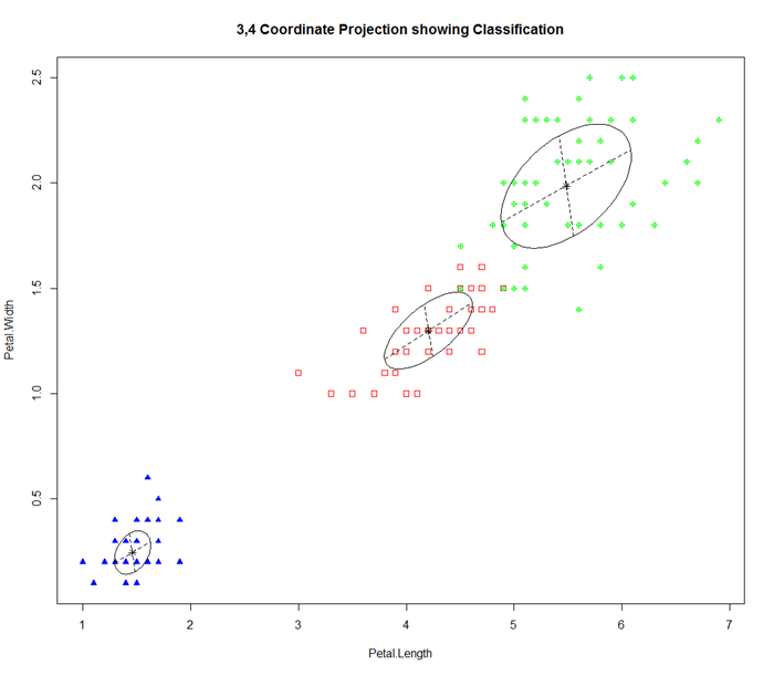
Density-based Cluster
In density based cluster, a cluster is extend along the density distribution. Two parameters is important: "eps" defines the radius of neighborhood of each point, and "minpts" is the number of neighbors within my "eps" radius. The basic algorithm called DBscan proceeds as follows
- First scan: For each point, compute the distance with all other points. Increment a neighbor count if it is smaller than "eps".
- Second scan: For each point, mark it as a core point if its neighbor count is greater than "minpts"
- Third scan: For each core point, if it is not already assigned a cluster, create a new cluster and assign that to this core point as well as all of its neighbors within "eps" radius.
Here is an example of doing DBscan in R
> library(fpc)
# eps is radius of neighborhood, MinPts is no of neighbors
# within eps
> cluster <- dbscan(sampleiris[,-5], eps=0.6, MinPts=4)
> plot(cluster, sampleiris)
> plot(cluster, sampleiris[,c(1,4)])
# Notice points in cluster 0 are unassigned outliers
> table(cluster$cluster, sampleiris$Species)

setosa versicolor virginica
0      1          2         6
1      0         13         0
2     12          0         0
3      0          0         6

Although this has covered a couple ways of finding cluster, it is not an exhaustive list. Also here I tried to illustrate the basic idea and use R as an example. For really large data set, we may need to run the clustering algorithm in parallel. Here is my earlier blog about how to do K-Means using Map/Reduce as well as Canopy clustering as well.
2 comments:
Excellent article!
Hey,
Thanks for this. I've followed it and found it really interesting. Just a quick comment.
In the Multi-Gaussian with Expectation-Maximization example the plot causes an error formal argument "data" matched by multiple actual arguments.
To solve it you can change the plot command to plot(mc, what=c('classification'), dimens=c(3,4))
Post a Comment